Linear Regression Model Selection (feat. Geomertry)

Linear Regression Fails with Many Predictors

Linear regression is powerful in that it allows us "humans" to understand what is happening in the model and how the model reasoned to make a prediction. This is because Linear regression essetially outputs a linear equation like below:

$$y = \beta_0 + \beta_1 x_1 + \beta_2 x_2 + \cdots + \beta_n x_n$$

where $y$ is the output variable, $x_1, x_2, \cdots, x_n$ are the input variables, and $\beta_0, \beta_1, \cdots, \beta_n$ are the coefficients of the input variables.

However, it gets complicated when we are trying to introduce many input variables, sometimes more variables than the number of observed samples. In such case, simple linear regression model that uses all the input variables (Ordinary Least Squares) can overfit the data and output poor results.

Model Selection with Ridge and Lasso

To remedy cases where we have many input variables, there are mainly three methods we can use to create another linear regression model.

1. Forward and Backward Selection: This method selects the best subset of input variables that can explain the output variable. It is a brute-force method that tries all possible combinations of input variables and selects the best subset.

2. Shrinkage method: This method shrinks the coefficients of the input variables to zero. This method is useful when we have many input variables and we want to select only the important variables. There are two types of shrinkage methods: Ridge and Lasso.

3. Dimension Reduction: This method reduces the dimension of the input variables. This method is useful when we have many input variables and we want to reduce the number of variables. One example of this would be Primary Component Analysis (PCA).

In this post, we will focus mainly on shrinkage method and introduce them not as how it is normally explained but by using geometric images to explain what is happening in them.

Brief Introduction of Ridge and Lasso

To first understand Ridge and Lasso, one should have a good understanding of Ordinary Least Squares, which is the most basic version of linear regression model.

The ultimate goal of Ordinary Least Squares is to find the coefficients ($\beta_0, \beta_1, \cdots, \beta_n$) of the predictors that make the residual sum of squares (RSS) to 0. The Residual sum of squares is calculated as below:

$$RSS = \sum_{i=1}^{n} (y_i - \hat{y}_i)^2$$

where $y_i$ is the actual output value and $\hat{y}_i$ is the predicted output value.

Since OLS goal is just to minimize the difference between the actual and predicted output values, it can be said that OLS has the least bias.

OLS and MSE?

OK. Now frankly speaking, many already know MSE (Mean Squared Error) since it is a term that appears both in statistics and machine learning. But what is OLS? It seems that they are connected but how?

So Ordinary Least Squares (OLS) can be best understand when contrasted with other methods that have similar names. Other than OLS, there is also a a WLS which is Weighted Least Squares. So, both have least squares in their names and essentially they compare between the actual and predicted values whose difference is squared for later minimization. However, WLS applys weights to the squared differences to specific samples. Essentially its goal is to minimize the weighted sum of squared differences:

$$Minimize \sum_{i=1}^{n} w_i(y_i - \hat{y}_i)^2$$

where $w_i$ is the weight applied to the $i$-th sample.

On the other hand, OLS does not apply any weights to the squared differences. It just tries to minimize the sum of squared differences:

$$Minimize \sum_{i=1}^{n} (y_i - \hat{y}_i)^2$$

In fact, the 'Ordinary' in OLS means that it does not apply any weights to the squared differences. It just tries to minimize the sum of squared differences. (For your information $\sum_{i=1}^{n}(y_i - \hat{y}_i)^2$ is also called the Residual Sum of Squares (RSS).)

So how does Mean Squared Error (MSE) come into play? Well, MSE is essentially the average of the squared differences between the actual and predicted values. So it can be said that MSE is the average of the RSS. Thus, it can be said that OLS is the method that tries to minimize the MSE.

$$MSE = \frac{1}{n} \sum_{i=1}^{n} (y_i - \hat{y}_i)^2$$

Calculation of Bias and Variance

Allright, so we have been told that OLS has the least bias among linear regression models. Let us talk about the bias and variance of it.

Now when talking about models, bias and variance are two keywords that always show up. Essentially in predictive models, there is always a bias and variance tradeoff. The most famous image that explain both bias and variance is the image below:

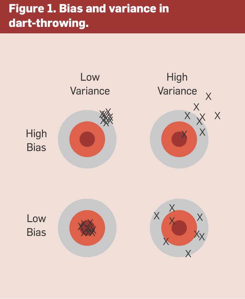
In the image, the bullseye is the target. The lower the variance, the denser the shots are to each other (regardless of its proximity to the bullseye). The higher the bias, the more offset the shots are from the bullseye. In linear regression, it is a common practice to find a model that has the least bias and variance, which is in fact difficult due to the tradeoff that exists between them.

Now how to calculate the variance is relatively easy. It is the standard deviation of the predicted values themselves. In calculating the variance, there is no need to rely on the actual values. The variance can be calculated as below:

$$Var(\hat{y}) = E[(\hat{y} - E[\hat{y}])^2]$$ $$Var = \frac{1}{n} \sum_{i=1}^{n} (\hat{y}_i - E[\hat{y}])^2$$

where $E[\hat{y}]$ is the expected value of the predicted values.

As you can see, there is no need to rely on the real observed $y$ values. The variance can be calculated just by using the predicted values.

However, bias is a bit more complicated. Bias is the difference between the expected value of the predicted values and the actual values. Thus, it requires us to have our observed $y$ values. The bias can be calculated as below:

$$Bias(\hat{y}) = E[\hat{y}] - y$$ $$Bias = \frac{1}{n} \sum_{i=1}^{n} (\hat{y}_i - y_i)$$

where $y$ is the actual output values.

OLS has the least bias?

So, why is OLS said to have the least bias in a mathematical perspective? Let us remember that OLS attempts to minimize the below function

$$RSS = \sum_{i=1}^{n} (y_i - \hat{y}_i)^2$$

For exploaratory purposes, we can safely say that minimizing $RSS$ is the same as minimizing $MSE$ which is

$$MSE = \frac{1}{n} \sum_{i=1}^{n} (y_i - \hat{y}_i)^2$$

In fact, if we calculate the MSE in $E$ term it is,

$$MSE = E[(y - \hat{y})^2]$$

which eventually leads to the interpretation of MSE as a function of bias and variance. You may look at how the below function is derived through this link

$$MSE = Bias^2 + Var + \sigma^2$$

where $\sigma^2$ is the irreducible error.

If assumptions on the linear model are held, then the bias of the OLS model is 0 according to the Gauss-Markov theorem. The assumptions are 1) the model is linear in the parameters, 2) the errors of residuals are independent and identically distributed, 3) the errors are normally distributed (mean should be 0), and 4) the errors have a constant variance. If these assumptions are held, then the OLS model has the least bias. The specifics of Gauss-Markov theorem can be found in this link. But just to give you a brief overview, In the final equation of the theorem, the OLS model shows that the mean of the estimated coefficients is equal to the true coefficients.

$$E[\hat{\beta}] = \beta$$

If the above is held, the the model can be said to have a bias of 0.

Ridge Regression

We have come a long way to really discuss about Ridge Regression and Lasso Regression. So Ridge Regression and Lasso manipulates the bias and variance of the model by adding a penalty term to the OLS model. The penalty term is added to the original RSS and the goal of the Regression model changes to minimizing the below function:

$$Minimize \sum_{i=1}^{n} (y_i - \hat{y}_i)^2 + \lambda \sum_{j=1}^{p} \beta_j^2$$

So as you can see here, a new term $\lambda \sum_{j=1}^{p} \beta_j^2$ is added to the RSS function. This term is called the penalty term. The penalty term is the sum of the squares of the coefficients of the input variables. The $\lambda$ is the hyperparameter that controls the strength of the penalty term. If $\lambda$ is 0, then the penalty term is 0 and the model is the same as the OLS model. If $\lambda$ is very large, then the penalty term is very large and the coefficients of the input variables are shrunk to 0.

In easy words, Ridge Regression introduces a constraint budget that the RSS should be operated within. Remind yourself that this is a constraint! The whole point of Ridge Regression is to find the coefficients ($\beta_0, \beta_1, \cdots, \beta_n$) that minimize the RSS while keeping the sum of the squares of the coefficients within the budget. This is why Ridge Regression is also called L2 regularization.

This is in fact an optimization problem! We are given a budget and we need to find the point where the RSS is minimized while keeping the sum of the squares of the coefficients within the budget.

Let us understand this easily using geometry. For simplifying the problem let us imagine a two predictor linear regression model. This model will be expressed as below:

$$y = \beta_0 + \beta_1 x_1 + \beta_2 x_2$$

Our goal in Ridge Regression is to find the coefficients ($\beta_0, \beta_1, \beta_2$) that minimize the RSS while keeping the sum of the squares of the coefficients within the budget. But before we go into plotting lines and curves to understand how Ridge Regression works, let us first understand OLS in a geometric perspective.

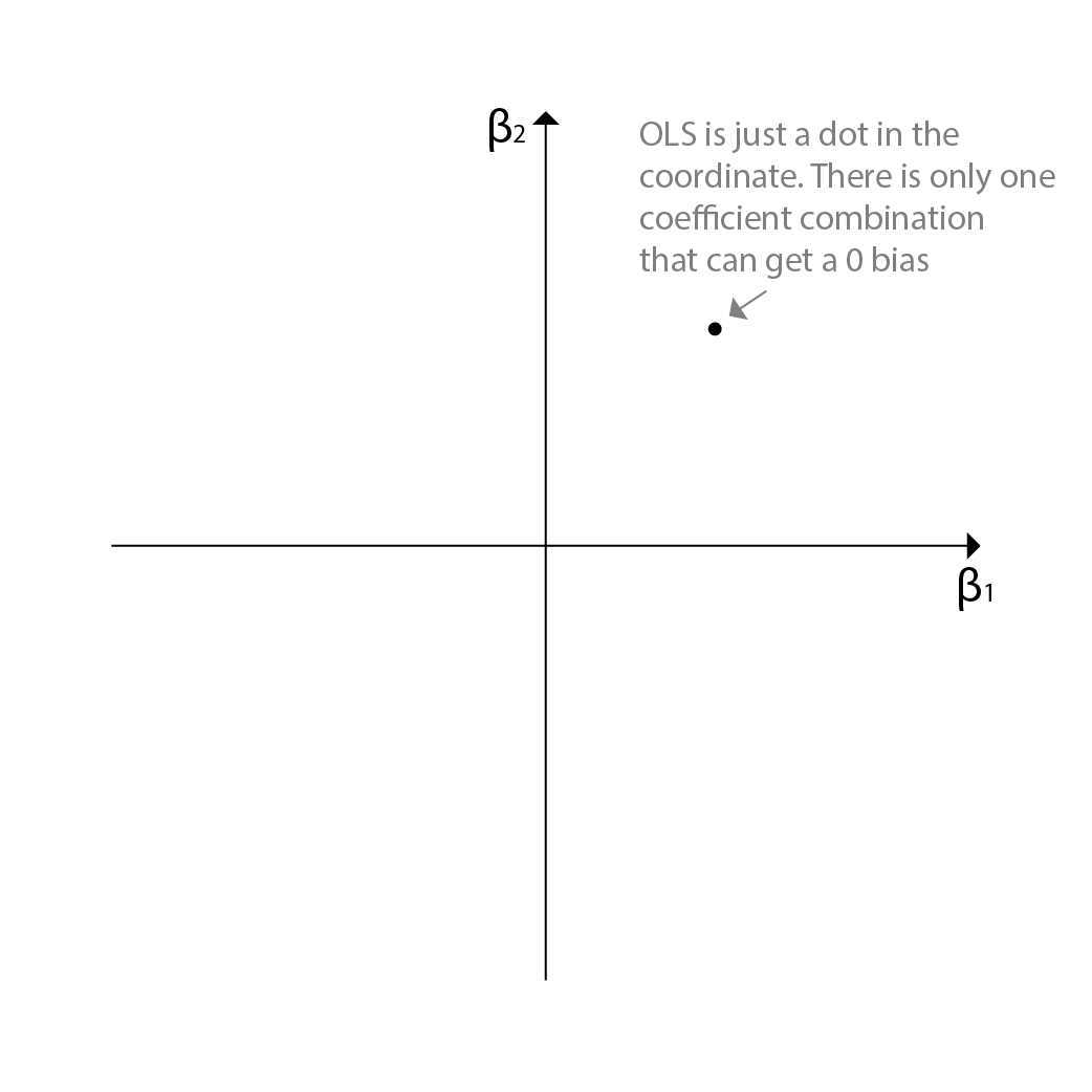
OLS in a Geometric Perspective

Since we have a two predictor linear regression model, we can plot the combination of all the coefficients into a 2d plane. OLS model will give us only one single combination in the 2d plane, since there is only one combination that can minimize the RSS in the linear regression model. This is the combination that is closest to the actual output values.

Ridge Regression in a Geometric Perspective

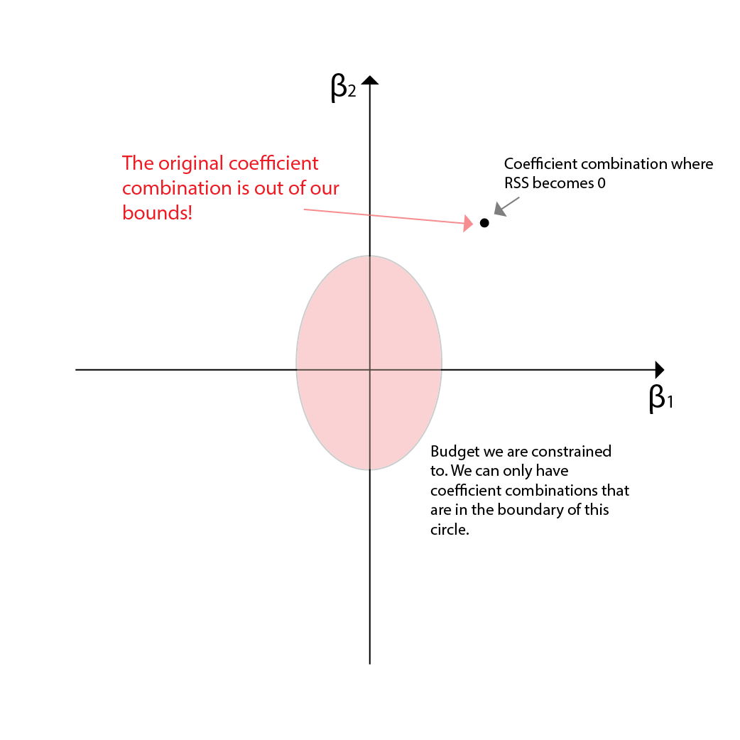
OLS was relatively easy to understand. Now how about Ridge Regression? First remind that Ridge Regression is minimizing the RSS within a fixed budget. Thus it is an optimization probelm. Our budget can be depicted as an area in the 2d plane. Plus, since our ridge regression is a square of the coefficients, the budget area will be a circle.

Now the dynamic variable is only the RSS. We need to sacrifice RSS to find the right coefficient combination that is within the budget (=the point should fall in the area of the circle). As we sacrifice more and more of the RSS, the coefficients will change. What happens if we sacrifice RSS? The RSS will be a value higher than 0 and thus, many coefficients can satisfy to meet such RSS. For instance for a RSS=1, the coefficient combinations will be shown as a line in the 2d plane. All combination points on the line will have a RSS of 1.

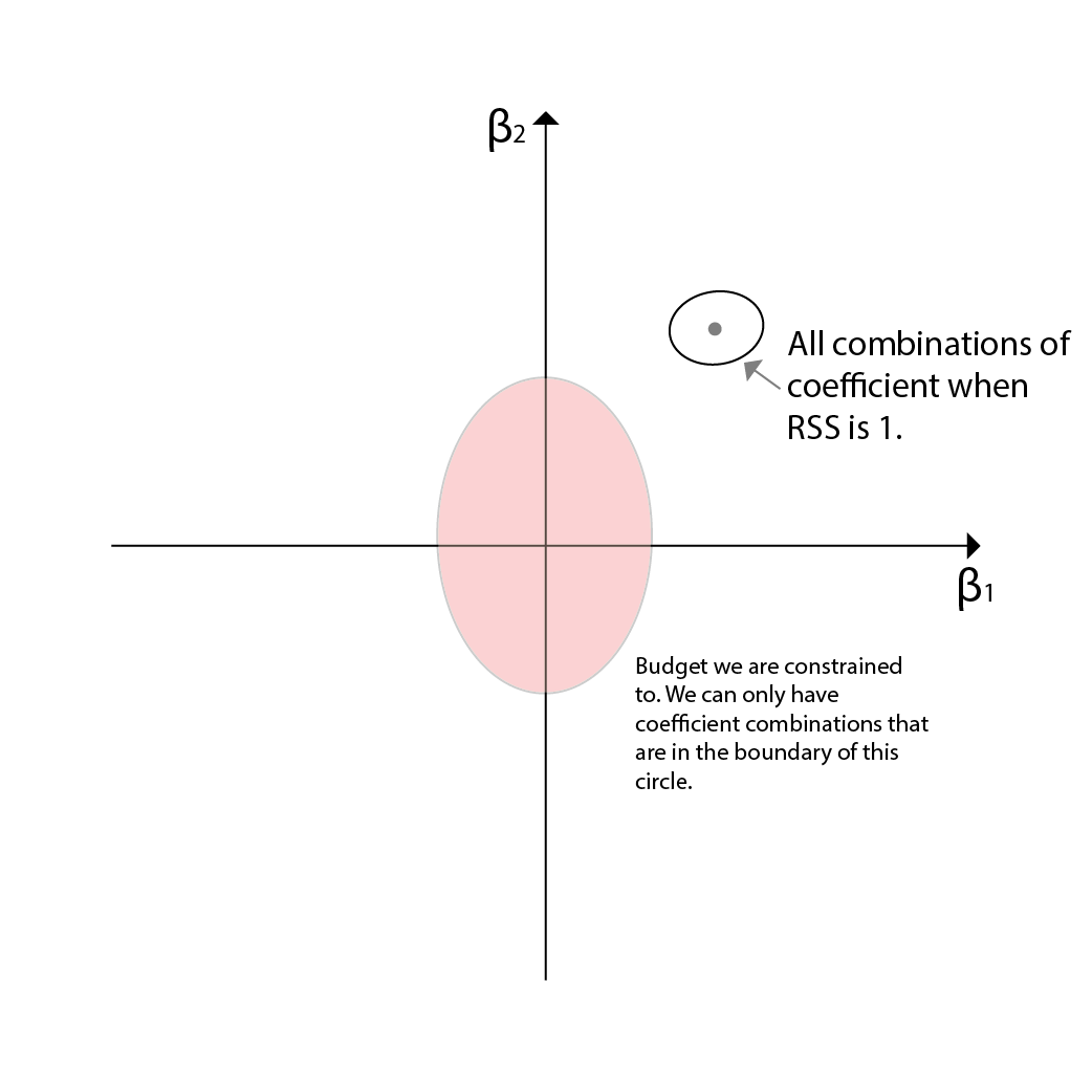
However, remember that though the coefficients can get larger than the original RSS=0 coefficients, we only care about the smaller coefficients since they are the ones that are highly likely to be met in the budget area. This is why Ridge Regression is also called a shrinkage method. The coefficients are shrunk to 0 to find the right combination that is within the budget. Since none of the points in RSS=1 line is within the budget, we need to continue sacrificing the RSS to find the right combination.

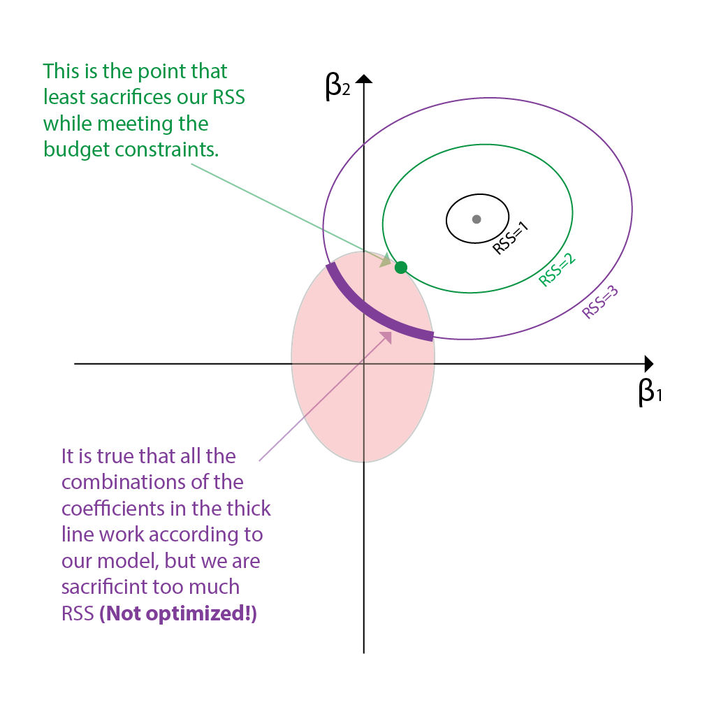
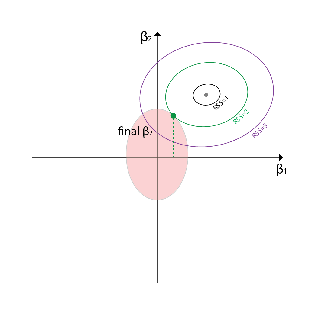
As we continue to sacrifice the RSS, the line of possible combinations of coefficients will be larger and larger. Eventually, we will find the right combination that is within the budget. This is the combination that minimizes the RSS while keeping the sum of the squares of the coefficients within the budget. Since both the area and our line are ellipses, the combination that is the best combination will be the point where both ellipses intersect to each other.

Though we can sacrifice the RSS more and find more combinations that can fit within the boundaries, we have to remember that this is an optimization problem. Thus, the combination that is the best is the one that minimizes the RSS while keeping the sum of the squares of the coefficients within the budget. This is the combination that is the closest to the actual output values. This is in fact the point where the Ridge Regression model stops its exploration and outputs the coefficients.

Lasso Regression in a Geometric Perspective

Now how is Lasso Regression expressed in the coordinates. First, we should remind ourselves how lasso regression is different from ridge regression. Lasso regression is also a shrinkage method, but it uses the sum of the absolute values of the coefficients as the penalty term. This is why Lasso Regression is also called L1 regularization.

The penalty term of Lasso Regression is expressed as below:

$$Minimize \sum_{i=1}^{n} (y_i - \hat{y}_i)^2 + \lambda \sum_{j=1}^{p} |\beta_j|$$

Now the penalty term is different from the Ridge Regression. Thus the budget area will not be shown as an ellipse but a rectangular. Everything else is the same. We need to sacrifice RSS untill there is a point that is within the budget area.

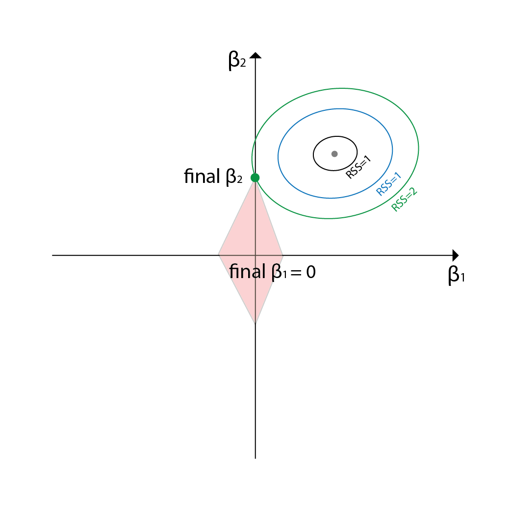
If you see the intersecting point, there is an interesting thing that happens. The Lasso Regression model can output a combination that has some of the coefficients to be 0. This is due to the shape of the budget area. In Ridge regression, the budget area was an ellipse, and thus it is hihgly unlikely for the intersecting points to end up on the axes. However, in Lasso Regression, the budget area is a rectangle, and thus it is highly likely for the intersecting points to end up on the axes. Due to this, Lasso Regression can output a combination that has some of the coefficients to be 0.

Conclusion

This is the end of the explanation of Ridge and Lasso Regression in a geometric perspective. I hope that this explanation was helpful in understanding how Ridge and Lasso Regression works. I would like to thank Professor Soroush Saghafian for helping me understand this topic!

Reference

1. An Introduction to Stastistical Learning