VAE the basics

What is VAE for?

Variational Autoencoder (VAE) is known to be a more advanced Autoencoder (AE). The main difference between AE and VAE is that VAE has an additional statistical feature added to it in the middle. Both AE and VAE network inputs multi-dimensional data and outputs a multi-dimensional output that has a high resemblance to the inputted data. Thus, it means that AE and VAE are networks that try their best to output the same data that was initially inputted. How they train the parameters for making such output is through an encoder and decoder network, where the encoder tries to compress the multi-dimensional input into smaller data and make the decoder recreate(=reconstruct) the image with that compressed data. In the AI realm, this compressed data is called a vector in a latent space.

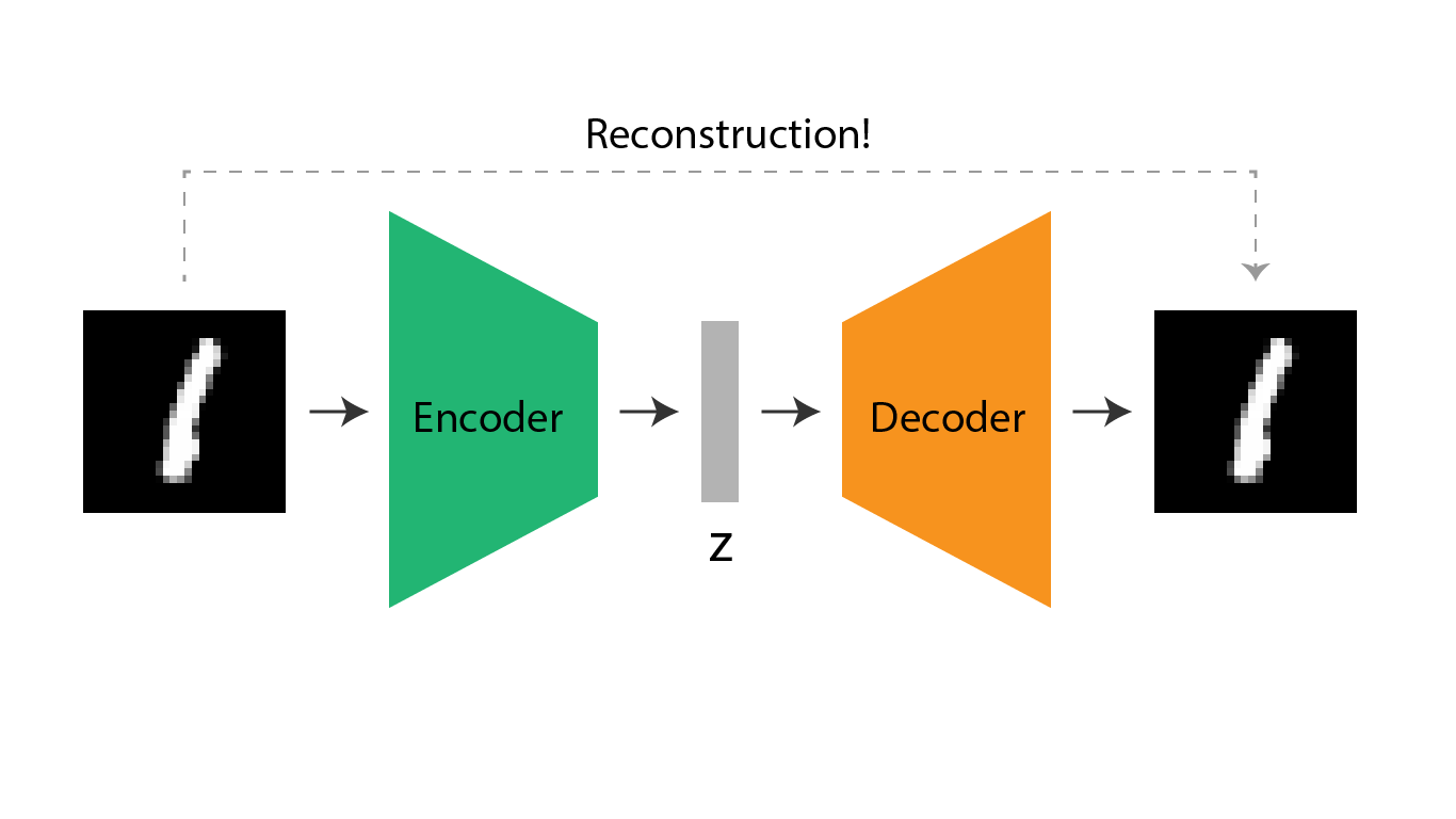
Though AE and VAE have similar structures, their purposes differ. While AE's main focus is on the encoder, the VAE's main focus is on the decoder. This means that AE's purpose is to compress the multi-dimensional data into a compressed vector while VAE's purpose is to generate images. For instance, AE can be mainly used to create an image-based search system where every uploaded image goes through the encoder network to output a vector composed of numbers, which will be used to find similar images compared to a newly inputted image. VAE can be used for generative purposes such as generating a new image.

In this post, the main focus is to get a glimpse into how VAE works. As mentioned above, the feature that makes VAE more advanced compared to AE is that it has a statistical feature added in the middle of the network.

The additional statistical feature in VAE

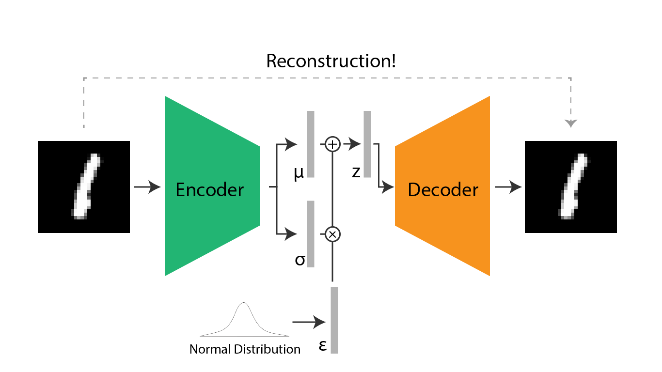
So I have previously said that there is an additional statistical feature in VAE. Why then is a probabilistic layer added to the latent space? VAE's purpose is to reconstruct well. Under the hood, VAE understands the inputted training samples as data with irregular and random noises. Thus a probabilistic layer on the latent space can filter out the noise that has not much to do with the inherent signal of the data.

In the VAE network, this probabilistic layer is implemented by extracting a μ vector and a σ vector, each representing the mean and standard deviation of the input data. In many practices, the VAE network is assumed to have a normal distribution, μ is 0 and σ is 1. Thus in the training process, while extracting two vectors, one for μ and one for σ, we must take measures to make the μ and σ follow the normal distribution.

I first was curious whether it is possible to extract the μ and σ of a multi-dimensional input. Was there a mathematical function to get the μ and σ of any encoded data? However, after looking through some codes, it became evident that there does not exist a specific mathematical approach to calculating the μ and σ. In most networks, μ and σ are simply vectors that go through a linear layer in the encoder network. It is the loss function's job to make the linear layers to make the two vectors the μ and σ of a normal distribution. The element that makes the two vectors into the μ and σ of a normal distribution is the KL divergence loss element, which is something that is discussed in the later paragraphs.

class Encoder(nn.Module):

    def __init__(self, input_dim, hidden_dim, latent_dim):
        super(Encoder, self).__init__()

        self.FC_input = nn.Linear(input_dim, hidden_dim)
        self.FC_input2 = nn.Linear(hidden_dim, hidden_dim)
        self.FC_mean  = nn.Linear(hidden_dim, latent_dim)
        self.FC_var   = nn.Linear (hidden_dim, latent_dim)

        self.LeakyReLU = nn.LeakyReLU(0.2)

        self.training = True

    def forward(self, x):
        h_       = self.LeakyReLU(self.FC_input(x))
        h_       = self.LeakyReLU(self.FC_input2(h_))
        mean     = self.FC_mean(h_)
        log_var  = self.FC_var(h_)
        return mean, log_var

As you can see in the above code, there are not any mathematical measures added to make mean and variance vectors.

Sampling a latent space vector

Now that we got a hang of the meaning of a probabilistic layer inside a VAE, it is now time to understand how the latent space vector is sampled. In short, how is a latent space vector, z, created through the extracted mean and variance vectors? The best method is to randomly choose a vector from the normal distribution represented by the mean and variance vectors. However, when a latent space vector, z, is created through such a process, there is no way the VAE model can update its parameters through backpropagation. The selection of a latent space vector through the statistical method is not differentiable.

Researchers instead introduced a new approach to create a latent space vector out of the mean and variance vector. What they did was simply use arithmetic operations to create a latent space vector. $z=\mu+\sigma*\epsilon$. $\epsilon$ here is a randomly chosen vector in a normal distribution. This method is called the Reparameterization Trick. The math behind this trick is very complex and I will not go into detail about the math.

Math behind VAE

For a neural network to train its parameters, a clear purpose of the model should be set. As mentioned above, the main goal of the VAE is to well reconstruct the original input through the decoder. Thus, if we say the parameters of the decoder network is $\theta$, our goal is to make the probability of x, original, maximum, $p_\theta(x)$. We use our latent space vector, z to accomplish this, so the function should take z into consideration. If we change the function to incorporate z, it is $\int p_\theta(z)p_\theta(x|z) \, dz$. The reason $p_\theta(x|z)$ appeared is because the combined probability of x and z can be represented as x|z. $\frac{p_\theta(x,z)}{p_\theta(z)} = p_\theta(x|z)$, which also means $p_\theta(x,z)=p_\theta(z)\times p_\theta(x|z)$. We know that $\int p_\theta(x,z) \, dz = p_\theta(x)$. In fact, $p_\theta(x|z)$ is the representation of the decoder network of VAE.

However, the problem is that the integral for $p_\theta(x|z)$ cannot be calculated(=intractable). In the context of integral, having that $p_\theta(x|z)$ means that we have to calculate the probability of x for all latent space vector z. Researchers thought that if $p_\theta(x|z)$ cannot be directly, why not find the posterior distribution, distribution of latent variables given the observed data, $p_\theta(z|x)$? In addition to escaping the burden of finding the $p\theta(x|z)$, since the VAE's job is to generate outputs that are highly similar to the inputted data, a well-structured latent space can ensure continuity and completeness. This is why a VAE necessitates the training of an encoder despite its main focus on the decoder.

Unfortunately, finding $p_\theta(z|x)$ is also not an easy task since finding $p_\theta(z|x)$ also necessitates a prior knowledge of $p_\theta(x)$. $p_\theta(z|x)=\frac{p_\theta(x|z)\times p_\theta(z)}{p_\theta(x)}$. Thus we need to accept the fact that we cannot find the $p_\theta(z|x)$ directly, but instead train an encoder network that is close to $p_\theta(z|x)$. The encoder network will be represented as $q_\phi(z|x)$.

So back to the original purpose of VAE. Our goal is to maximize the data likelihood, $p_\theta(x)$. Let us add a log to the value to make our calculations simple. $\log{p_\theta(x^{(i)})}$. i is a value from 1 to N, and N represents the number of input data. To make the calculation simple we make the value as Expectation, $E_{z \sim q_\phi(z|x^{(i)})}[\log p_\theta(x^{(i)})]$. Here, z follows the distribution of our encoder($q_\phi(z|x^{(i)})$). According to Bayes' rule, we can change the $p_\theta(x^{(i)})$ into $\log \frac{p_\theta(x^{(i)}|z)p_\theta(z)}{p_\theta(z|x^{(i)})}$. The following math is shown in the image below.

Bayes rule

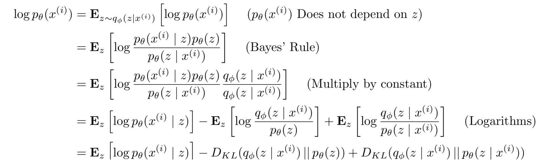
As shown in the image, in the end, we end up with three terms we need to consider when maximizing $\log{p_\theta(x^{(i)})}$. Unfortunately, since $p_\theta(z|x^{(i)})$ is intractable, the last KL term cannot be calculated. However, due to KL divergence outputting a result that is always >=0, we can kindly disregard this term. The initial two terms combined are called the Variational lower bound(=ELBO) in a VAE, and our goal is to maximize the ELBO. The first term in ELBO is related to the decoder network and the second term in the ELBO is related to the encoder.

What we need to find

Since loss functions are often expressed as minimizing the function. we can change the above expression into the loss function below

The first term has to do with reconstruction error, where it outputs the error to how much the $x_i$ was wrongly reconstructed, and the second term has to do with the regularization error, where it outputs the encoder's deviation from the normal distribution $p(z)$ (remember that we initially supposed the distribution of latent space vector z to be a normal distribution)

Analyzing the loss function terms

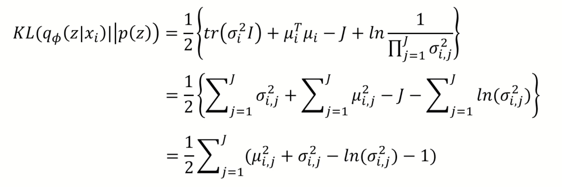
Minimizing the loss in regularization is done by the KLD operation for two distributions. Since the $p(z)$ was set to a normal distribution, the function is relatively simple (I will not discuss the specifics of how KLD is calculated)

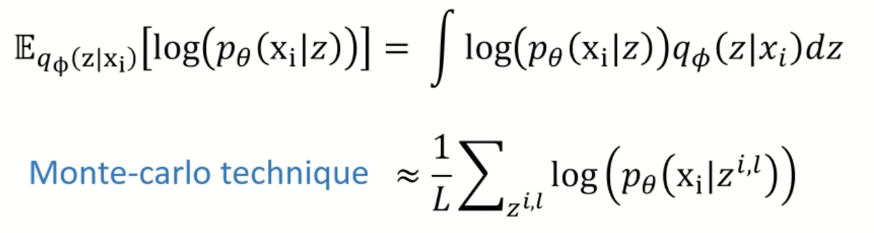
Minimizing the reconstruction error is a little bit more complex due to the necessity to take probabilities into consideration. For this purpose, the researchers used a Monte Carlo technique to simplify the calculation of integral. Also, the L was set to 1 to make the calculation even simpler, resulting in a reconstruction loss calculation to $\log(p_\theta(x_i|z^{(i)}))$

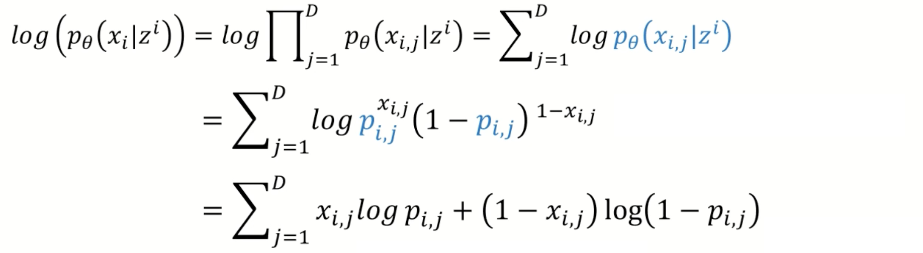
Now to further calculate $\log(p_\theta(x_i|z^{(i)}))$, the characteristic of the p should be determined. The probability can either follow a multivariate Bernoulli or a Gaussian distribution. In the case of bernoulli, $\log(p_\theta(x_i|z^{(i)}))$, the probabilities of each item in the $x_i$ should be multiplied. In logarithmic operation, multiplication can be considered as additions. Thus the below cross entropy can be calculated. By the way, $p_{i,j}$ is the decoder network output.

References

1. https://www.youtube.com/watch?v=GbCAwVVKaHY&list=LL&index=1
2. https://medium.com/tensorflow/variational-autoencoders-with-tensorflow-probability-layers-d06c658931b7
3. https://towardsdatascience.com/on-distribution-of-zs-in-vae-bb9a05b530c6
4. https://medium.com/analytics-vidhya/variational-autoencoders-explained-bce87e31e43e
5. https://sassafras13.github.io/ReparamTrick/
6. http://cs231n.stanford.edu/slides/2017/cs231n_2017_lecture13.pdf
7. https://jaan.io/what-is-variational-autoencoder-vae-tutorial/